Hierarchical polyphonic active inference in a 3D PyBullet environment

An embodied drone controller built around belief dynamics, scene interpretation, and future-scene reasoning

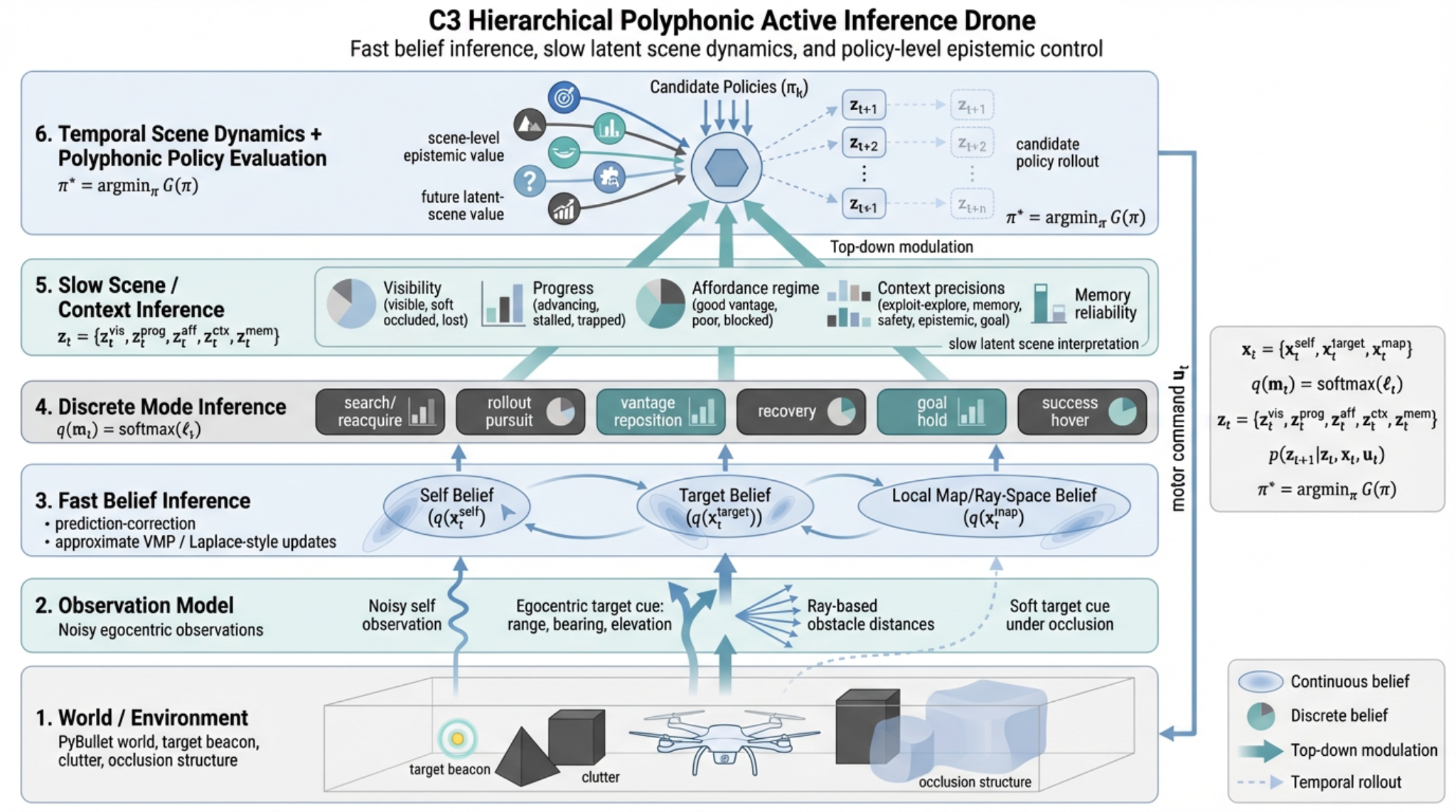
This project implements a drone agent that must reach a target beacon in a cluttered three-dimensional world under partial observability. The controller is not given simulator truth. Instead, hidden-state estimates are updated online from noisy self-observations, egocentric target cues, and ray-based obstacle sensing, and action is selected from those beliefs by a polyphonic control architecture whose pressures are modulated by a slower latent scene layer.

The system combines continuous belief updates, posterior-like behavioural mode arbitration, scene-level epistemic control, and temporal latent scene dynamics. In practice this allows the drone to remember the target under occlusion, distinguish poor vantage from genuine blockage, switch between exploration and exploitation, and choose actions partly for how they are expected to improve the future scene rather than only the immediate target distance.

PyBullet

Belief-state control

Egocentric sensing

Gaussian/Laplace filtering

Discrete mode inference

Temporal scene dynamics

Policy-level epistemics

Watch the demo See the architecture

Demonstration run of the current controller. The overlay shows the target belief, confidence, observation status, behavioural mode, and the slower scene/context variables that bias exploration, exploitation, and repositioning.

1152

control steps in the attached successful run

0.26 m

minimum distance to target achieved

538

steps with direct target visibility

concurrent control voices informing policy evaluation

Why this system is interesting

Many active inference demonstrations remain either highly discrete or unrealistically privileged. This system was designed to move beyond that. The drone inhabits a continuous 3D environment, receives only local noisy cues, and must reach a target while maintaining a coherent belief state through periods of occlusion, clutter, and changing line-of-sight geometry. The policy does not reduce to direct pursuit of a known coordinate.

The more distinctive feature is the organisation of uncertainty. The agent maintains a fast belief layer over self state, target state, and local obstacle structure; a discrete layer over behavioural modes; and a slower latent scene/context layer that summarises whether the world currently looks visible, soft-occluded, lost, advancing, stalled, trapped, open, or blocked. Candidate policies are then evaluated not only for target progress and safety, but also for how much they are expected to clarify and improve these higher-order latent scene variables over time.

In practical terms, the controller asks not only “where is the target?” but also “am I merely occluded, genuinely blocked, or stuck in a poor-vantage region?”, and then uses that answer to bias what it does next.

C3 hierarchical polyphonic active inference drone architecture diagram

System diagram of the full architecture, showing the world and observation interface, fast belief inference, discrete mode arbitration, slow scene/context inference, and temporal scene-aware policy evaluation.

Ball-and-stick view of the architecture

The simplified graph highlights the main dependency structure: observations feed fast beliefs; fast beliefs support mode inference; slower latent scene variables modulate what the controller trusts; and candidate policies are evaluated partly for how they are expected to improve future scene state.

System architecture

1. Observation interface

The simulator retains ground truth internally, but the controller sees only noisy observations generated from that truth.

noisy self pose, velocity and yaw cues
egocentric target observations: range, bearing, elevation
ray-based obstacle distances
soft target evidence when the beacon is broadly localised but occluded

2. Fast inferential layer

The first inferential layer converts observations into posterior summaries over hidden state.

self belief: mean and covariance over pose and motion state
target belief: mean, covariance, confidence and occlusion history
local map belief: ray-wise structure of nearby free space
diagnostics: variance traces, confidence, visibility, deadlock signals

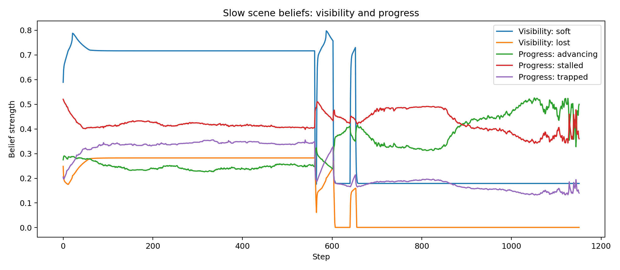
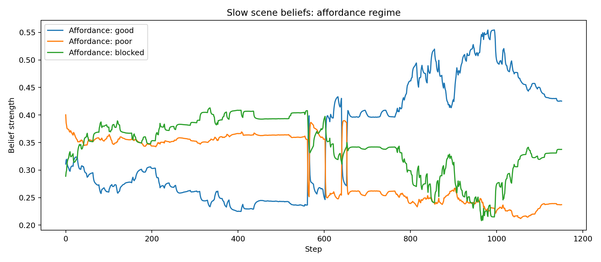
3. Slow scene and context layer

A slower latent layer interprets the current situation and predicts how that situation may evolve under different actions.

visibility regime: visible / soft-occluded / lost
progress regime: advancing / stalled / trapped
affordance regime: good-vantage / poor-vantage / blocked
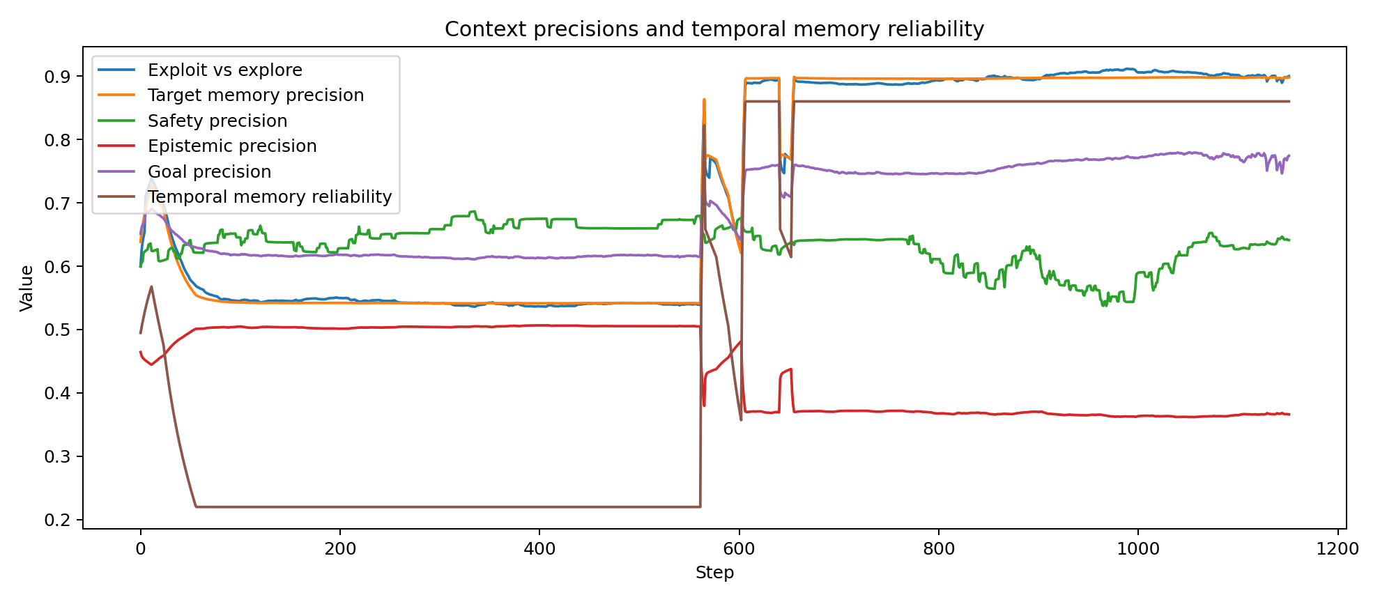
memory reliability and context precisions for exploration, safety and goal drive

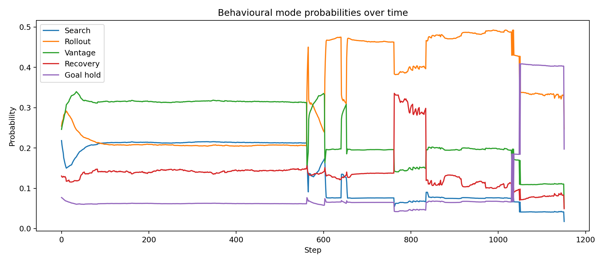
Behavioural arbitration

Action is not issued by a single monolithic controller. The system maintains posterior-like scores over a compact family of behavioural regimes, and the current regime is selected from those beliefs under the influence of target confidence, visibility, progress, local geometry, and scene/context interpretation.

search_reacquire: broad exploratory movement when target memory is weak or evidence is poor
efe_rollout: short-horizon forward evaluation of candidate controls under current beliefs
vantage_reposition: lateral or rotational manoeuvres that seek improved line of sight
recovery: conservative behaviour under poor local geometry or control deadlock
goal_hold: local stabilisation near the target
success_hover: terminal behaviour after the success condition is reached

These regimes are not intended as opaque labels. They are interpretable behavioural states that can be inspected, plotted, and related directly to changing beliefs over visibility, blockage, progress and target confidence.

Polyphonic control

Polyphony here means that candidate actions are evaluated under several concurrent behavioural pressures rather than one fixed objective. These pressures have their own effective precisions, and those precisions are shaped by the slower scene/context layer.

goal pressure: reduce target distance and alignment error
safety pressure: avoid collision-prone trajectories and cluttered local geometry
stability pressure: maintain altitude, heading and smooth control
epistemic pressure: reduce uncertainty over target and scene state
open-space pressure: prefer trajectories that improve geometry for future observations
scene-disambiguation pressure: clarify blocked versus poor-vantage interpretations
future-scene pressure: favour actions expected to lead into better latent scene regimes over time

The controller therefore does not merely chase the target. It can choose to move in ways that are temporarily suboptimal for distance reduction but useful for information gathering, line-of-sight recovery, or improvement of the future scene.

Step-by-step operation of the system

World state generates observations. The simulator computes the true drone pose, target position and obstacle geometry, but only noisy self cues, egocentric target cues, and ray-based obstacle distances are exposed to the controller.
Fast belief inference updates continuous hidden states. The filter updates posterior beliefs over self state, target state, and local map structure. This yields a target estimate with uncertainty and confidence rather than a privileged coordinate.
Behavioural mode beliefs are updated. The controller computes posterior-like scores over search, rollout, repositioning, recovery, hold and hover regimes using confidence, visibility, geometry, progress and deadlock cues.
Slow scene/context beliefs are inferred. A slower latent layer summarises whether the target is visible, soft-occluded or lost; whether progress is advancing, stalled or trapped; and whether the local geometry looks like good vantage, poor vantage or blockage.
Candidate policies are rolled forward. Short-horizon control sequences are imagined from the current belief state. Each is scored under the polyphonic objective, combining pragmatic, safety, stability, epistemic and future-scene terms.
Top-down modulation shapes what the controller trusts. The slow scene/context layer changes the effective weight of goal pursuit, exploration, safety and target-memory reliance without replacing the lower-level controller entirely.
The best action is executed and the cycle repeats. The selected motor command changes the world, which changes future observations, which in turn updates the next round of beliefs and policies.

Mathematical formulation

Fast hidden states

The fast latent state is factorised as

$$x_t = \{x_t^{\mathrm{self}},\; x_t^{\mathrm{target}},\; x_t^{\mathrm{map}}\}.$$

In the current implementation these are approximated by

$$x_t^{\mathrm{self}} = [p_x,p_y,p_z,v_x,v_y,v_z,\psi,\dot\psi],$$ $$x_t^{\mathrm{target}} = [g_x,g_y,g_z],$$ $$x_t^{\mathrm{map}} = [d_1,\dots,d_K],$$

where $d_k$ denotes the inferred obstacle distance along ray direction $k$.

Observations

The observation vector is

$$o_t = \{o_t^{\mathrm{self}},\; o_t^{\mathrm{target}},\; o_t^{\mathrm{rays}}\}.$$

It is generated from truth but consumed by the controller as noisy evidence:

$$o_t^{\mathrm{self}} = H_s x_t^{\mathrm{self}} + \omega_t^{s},$$ $$o_t^{\mathrm{rays}} = x_t^{\mathrm{map}} + \omega_t^{r},$$ $$o_t^{\mathrm{target}} = h(x_t^{\mathrm{self}},x_t^{\mathrm{target}}) + \omega_t^{g}.$$

Here $h(\cdot)$ returns egocentric range, bearing and elevation, with weaker soft observations when the target is broadly localised but occluded.

Continuous belief updates

The fast inferential layer maintains approximate Gaussian beliefs over self and target state,

$$q(x_t^{\mathrm{self}}) = \mathcal{N}(\mu_t^{s},\Sigma_t^{s}), \qquad q(x_t^{\mathrm{target}}) = \mathcal{N}(\mu_t^{g},\Sigma_t^{g}).$$

Beliefs are predicted forward under a local transition model and then corrected by precision-weighted prediction errors. A stylised form is

$$\mu_{t|t-1} = f(\mu_{t-1},u_{t-1}),$$ $$\Sigma_{t|t-1} = A_t\Sigma_{t-1}A_t^\top + Q,$$ $$\mu_t = \mu_{t|t-1} + K_t\big(o_t - h(\mu_{t|t-1})\big),$$ $$\Sigma_t = (I-K_tH_t)\Sigma_{t|t-1}.$$

For the target state, egocentric cues are reconstructed into world coordinates using the current self belief. Under prolonged soft occlusion, target confidence decays and covariance inflates, which prevents the agent from becoming spuriously certain about an unseen target.

Discrete mode beliefs

Behavioural arbitration is represented by a posterior-like belief over controller modes,

$$q(m_t) = \mathrm{softmax}(\ell_t),$$

where the logits $\ell_t$ depend on target confidence, visibility, local obstacle structure, progress, deadlock signals and proximity to target.

Slow scene/context state

The slower latent scene state is factorised as

$$z_t = \{z_t^{\mathrm{vis}},\; z_t^{\mathrm{prog}},\; z_t^{\mathrm{aff}},\; z_t^{\mathrm{ctx}},\; z_t^{\mathrm{mem}}\}.$$

These variables summarise visibility regime, progress regime, affordance regime, context precisions and target-memory reliability. They are updated from smoothed evidence and then used to bias control at the faster layer.

Temporal scene dynamics

The current controller also carries an explicit temporal model of how the slower scene variables evolve. In schematic form,

$$p(z_{t+1} \mid z_t, x_t, u_t).$$

This means the agent does not only infer what kind of situation it is currently in. It also predicts how visibility, progress, affordance and memory reliability are likely to change under different candidate actions.

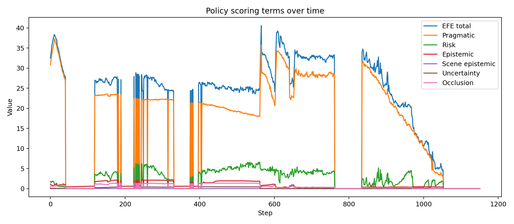
Polyphonic expected-free-energy-style scoring

For each candidate short-horizon control sequence $\pi_k$, the controller rolls the dynamics forward from the current belief state and computes a composite score:

$$G(\pi_k) = w_g J_{\mathrm{goal}}(\pi_k) + w_s J_{\mathrm{safety}}(\pi_k) + w_h J_{\mathrm{stability}}(\pi_k) + w_e J_{\mathrm{epistemic}}(\pi_k) + w_o J_{\mathrm{open}}(\pi_k) + w_d J_{\mathrm{scene}}(\pi_k) + w_f J_{\mathrm{future}}(\pi_k).$$

Representative terms are

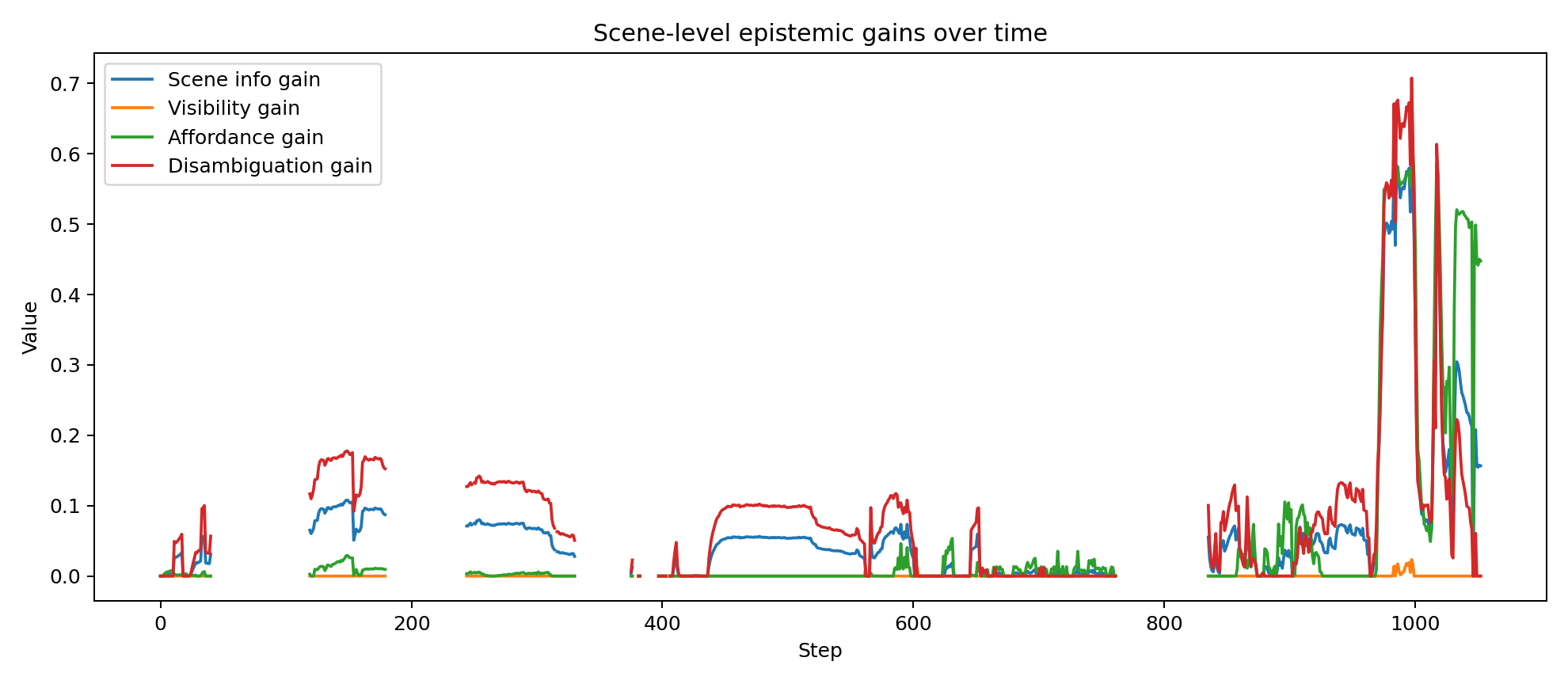
$$J_{\mathrm{goal}}(\pi_k) \approx \mathbb{E}_{q}[\|p_t-g_t\|],$$ $$J_{\mathrm{safety}}(\pi_k) \approx \mathbb{E}_{q}[\phi(d_{\min})],$$ $$J_{\mathrm{epistemic}}(\pi_k) \approx \mathrm{tr}(\Sigma_{t+H}^{g}) + \lambda_{\mathrm{occ}} C_{\mathrm{occ}}(\pi_k),$$ $$J_{\mathrm{scene}}(\pi_k) \approx - I_{\mathrm{scene}}(\pi_k),$$ $$J_{\mathrm{future}}(\pi_k) \approx - V_{\mathrm{future-scene}}(\pi_k).$$

Scene-level epistemic and future-scene value

The distinctive feature of the current controller is that epistemic value is not limited to target localisation. The controller also estimates whether an imagined action sequence is likely to clarify the latent scene state and improve the future scene trajectory.

$$I_{\mathrm{scene}}(\pi_k) \approx \Delta H\big(z_t^{\mathrm{vis}}\big) + \Delta H\big(z_t^{\mathrm{aff}}\big) + \lambda_{\mathrm{dis}}\,\Delta D_{\mathrm{blocked\;vs\;poor}},$$

$$V_{\mathrm{future-scene}}(\pi_k) \approx \mathbb{E}\big[\text{visibility improvement} + \text{progress improvement} + \text{affordance improvement} - \text{future scene uncertainty}\big].$$

Intuitively, policies are favoured when they are expected to improve visibility, disambiguate blocked corridors from poor vantage points, preserve useful target memory, and move the agent into a better latent scene over future steps.

Free-energy interpretation

The system can be read in standard active inference terms. The fast layer approximately minimises a variational free energy over hidden state,

$$F[q] = \mathbb{E}_{q(x_t)}\big[\ln q(x_t) - \ln p(o_t,x_t\mid u_{1:t-1})\big],$$

while action is selected by approximately minimising a structured expected-free-energy surrogate,

$$\pi^* = \arg\min_{\pi} G(\pi).$$

The implementation is intentionally lightweight rather than a full symbolic factor-graph engine, but it preserves the core active inference logic: actions are chosen for pragmatic value, safety, uncertainty reduction and future evidence, all conditioned on an evolving belief state rather than direct access to truth.

Implementation sketch

env/ drone.py # drone body and world dynamics sensing/ raycast_sensor.py # local obstacle sensing observation_model.py # noisy self and target observations belief/ belief_state.py # continuous, discrete and slow scene beliefs vmp_filter.py # approximate filtering and scene updates control/ autopilot.py # polyphonic controller and mode arbitration utils/ logging_utils.py # structured logs and overlays main.py # truth → observations → beliefs → action

The key engineering decision is that the controller never consumes simulator truth directly. Truth exists only to generate observations. This separation forces the policy to operate on beliefs, and it is the reason the system behaves like an inferential controller.

Control loop

for each timestep t: truth_state = simulator.read_state() observations = observation_model.sample(truth_state) belief_state = vmp_filter.step(belief_state, observations, previous_action) command, diagnostics, voice_info = controller.compute_command(belief_state) simulator.apply(command) logger.log(truth_state, observations, belief_state, diagnostics)

Observed behaviour

The drone successfully reaches the target while transitioning through a mixture of exploratory search, short-horizon rollout, local repositioning and target-hold behaviour. Logged summaries show:

successful target reach with minimum target distance of approximately 0.26 m
1152 total control steps with a healthy balance of exploratory and exploitative regimes
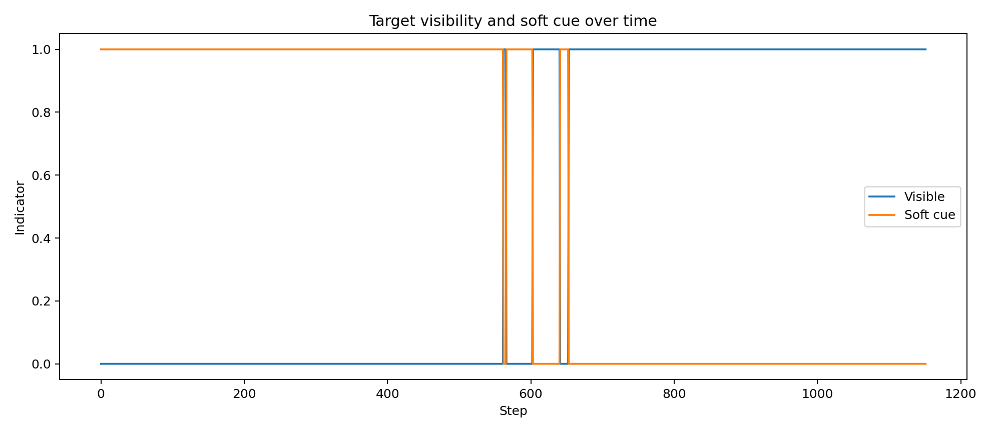
substantial time in both direct visibility and soft occlusion rather than trivial straight-line pursuit
non-zero scene-level epistemic and future-scene terms during policy evaluation
context variables that remain adaptive rather than collapsing into permanent search or permanent exploitation

What this demonstrates

This project shows that a relatively compact controller can integrate continuous latent-state estimation, discrete behavioural inference, slower contextual scene interpretation, and temporal scene-aware policy evaluation in a single embodied agent.

Run diagnostics and temporal traces

Because the controller is belief-based and explicitly hierarchical, its internal state can be inspected over time rather than inferred only from visible behaviour. The plots below were generated from the attached successful run and show how target confidence, behavioural arbitration, scene beliefs, contextual precisions, and policy-level epistemic terms evolve across the trajectory.

These traces are useful for validating that the system is doing something mechanistically meaningful: confidence rises and falls with evidence quality, mode probabilities shift between search and exploitation, scene beliefs respond to occlusion and progress, and the epistemic and future-scene terms become active at behaviourally relevant moments.

Target tracking and confidence over time

Target tracking and confidence. Distance to target, raw confidence, effective confidence, and target variance trace across the run.

Behavioural mode probabilities over time

Behavioural mode arbitration. Posterior-like probabilities over search, rollout, vantage reposition, recovery, and goal-hold.

Scene visibility and progress beliefs over time

Slow visibility and progress beliefs. The slower scene layer tracks whether the target is softly occluded or lost, and whether the agent is advancing, stalled, or trapped.

Affordance regime. Beliefs over good vantage, poor vantage, and blocked local geometry.

Context precisions and memory reliability over time

Context precisions. Exploit-explore balance, target-memory precision, safety precision, epistemic precision, goal precision, and temporal memory reliability.

Policy scoring terms. Decomposition of the expected-free-energy-style objective into pragmatic, risk, epistemic, scene-level, uncertainty, and occlusion terms.

Scene-level information gain. Visibility gain, affordance gain, and blocked-vs-poor-vantage disambiguation gain under candidate policies.

Target visibility and soft cue timing over time

Observation quality over time. When the target is directly visible versus only softly observed under occlusion.