Active Inference

What is active inference, and how is it different from other AI?

Active inference is a way of building intelligent systems that starts from a simple but powerful idea: an agent should not just react to the world, or chase rewards, but continually build predictions about the world and then update itself, and act, to reduce the mismatch between what it expects and what it senses.

Put differently: rather than treating perception, learning, and action as separate problems, active inference tries to explain them as parts of the same loop.

Start simple Jump to the maths Related consulting work

The simple version Deeper intuition A concrete example The maths Compared with other AI Figures & visualisations

Imagine a robot moving around a room looking for an object.

A lot of AI is framed in one of two ways. Either the system learns to map inputs to outputs, or it learns which actions tend to produce rewards.

Active inference starts somewhere else. It says the agent should build an internal model of the world, use that model to predict what it ought to sense next, and then reduce the gap between prediction and reality.

In that sense, the agent is not just reacting to the world. It is constantly trying to make sense of it, and acting so that what it senses becomes less surprising.

When there is a mismatch, two things can happen:

the agent can update its beliefs about what is going on, or
it can act to change what happens next.

That is the key move. Perception and action are not really separate. They are two ways of reducing prediction error.

Very short version: active inference says intelligent behaviour can emerge from a system that continually predicts, checks those predictions against reality, and updates beliefs or actions to reduce the mismatch.

At any moment, an agent does not directly observe the hidden causes of the world. It does not observe “where the object really is” in any perfect sense. It observes data: pixels, distances, touch signals, sound, motion cues, and so on.

So the agent has to infer the hidden state of the world from those observations. That is the perceptual part. But because the agent is embodied, it can also move, sample the world differently, and place itself somewhere new. That is the action part.

Active inference ties these together. The agent carries around beliefs about:

what state the world is in
how states generate observations
how actions change states over time
which outcomes it expects or prefers to encounter

Those beliefs are usually probabilistic. Not “the object is exactly here”, but “it is probably here, with some uncertainty”. That matters because uncertainty is not a minor detail. It changes behaviour.

When uncertainty is high
the agent is naturally pushed toward information-gathering behaviour: looking, moving, sampling, checking.

When beliefs are strong
the agent can act more decisively, because it has a sharper internal picture of what is going on.

This is one reason active inference is appealing. Exploration is not something awkwardly added later. It falls out of the same principle as perception and action.

Suppose we have a robot in a room. Its task is to find an object, grasp it, and return home.

A reward-based system might be told something like: “get points for approaching the object; get more points for returning home with it”.

In active inference terms, we can frame the problem differently. The robot has beliefs about where it is, where the object might be, whether the object has been grasped, and what observations it should receive if those beliefs are correct.

Early on, it may have a very uncertain belief about the object location. That pushes it toward exploratory actions. Once evidence accumulates, beliefs sharpen. After grasping, the preferred future changes: now the “good” predicted outcomes are those consistent with being back at home while retaining the object.

Before grasping: reduce uncertainty, find the object, bring observations in line with “the object is out there and can be reached”.

After grasping: bring observations in line with “I am back at home, holding the object”.

This is a useful way to think about active inference. It is not magic but a concrete control-and-inference scheme where goals, uncertainty, state estimation, and action selection are all written in the same language.

The central quantity is variational free energy. You can think of it as a tractable quantity the agent can minimise in place of surprise itself.

Core objective

\[ F[q] = \mathbb{E}_{q(s)}\left[\ln q(s) - \ln p(o, s)\right] \]

Here, o are observations, s are hidden states, p(o,s) is the generative model, and q(s) is the agent’s approximate posterior belief over states.

In practice, this quantity can be unpacked in a way that is often more intuitive:

Accuracy–complexity form

\[ F \approx \text{complexity} - \text{accuracy} \]

So a good model explains the data well, but without becoming needlessly complicated.

Minimising free energy therefore does two jobs at once. It improves the fit to sensory data and regularises the beliefs used to explain those data. This is why active inference is closely tied to variational Bayesian inference.

For action, the relevant quantity is expected free energy, which scores possible future policies.

Expected free energy

\[ G(\pi) = \mathbb{E}_{q(o, s \mid \pi)} \big[\ln q(s \mid \pi) - \ln p(o, s \mid \pi)\big] \]

A policy \pi is a candidate course of action. The agent evaluates policies by asking what sorts of outcomes and uncertainties they are expected to generate.

A common and very useful decomposition is that expected free energy captures both:

risk — whether future outcomes are inconsistent with preferred outcomes
ambiguity — whether future observations are likely to remain uninformative

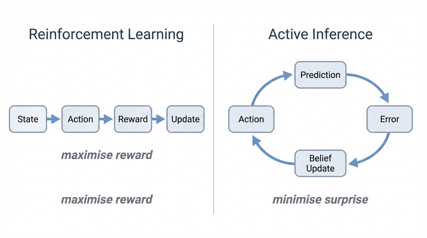
That means active inference naturally balances exploitation and exploration. The agent seeks outcomes it prefers, but it also values information when uncertainty is high.

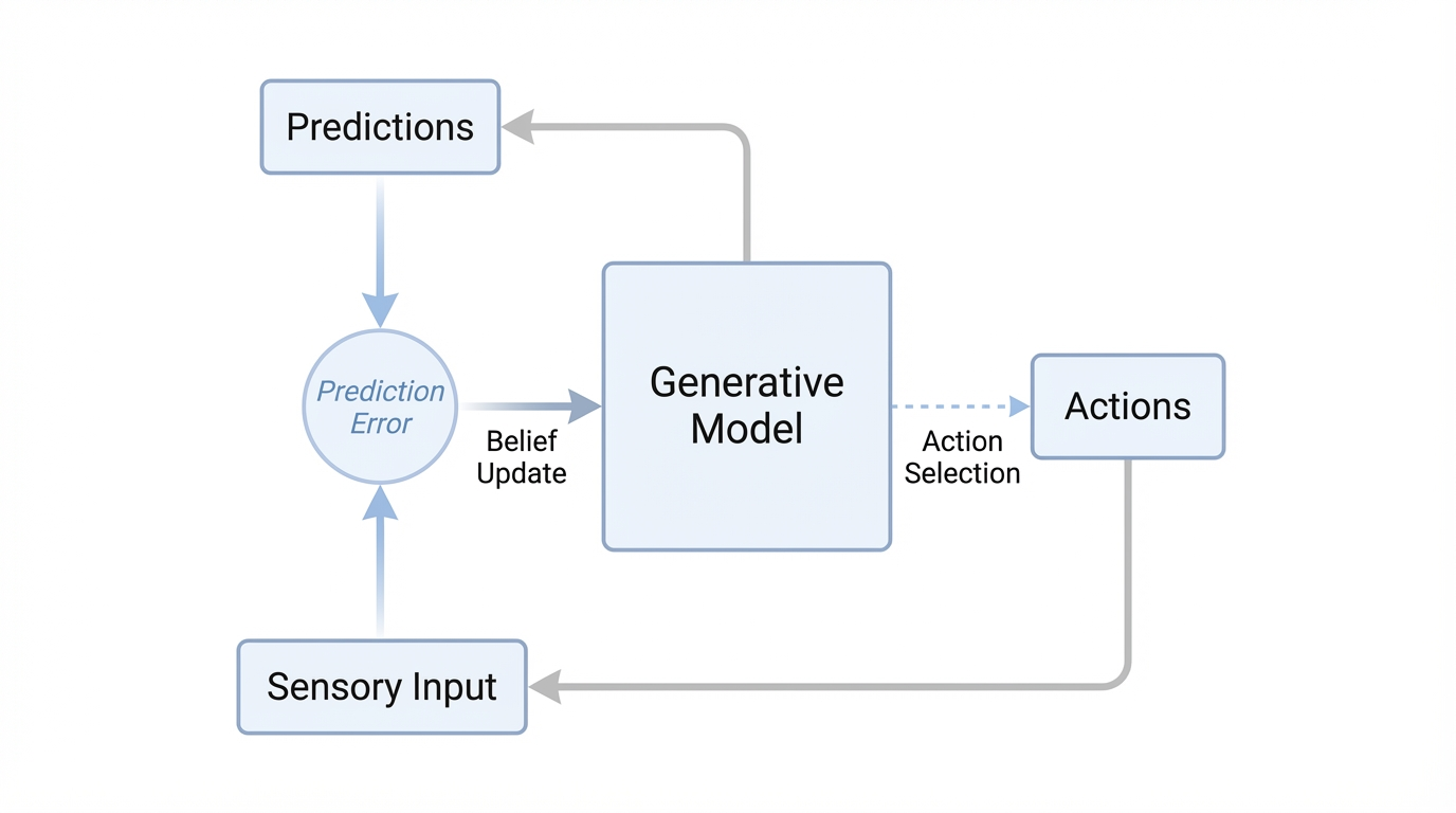
The important intuition: the same formalism that supports perception also supports planning. The agent is not switching between one system for inference and another for decision-making. It is using one probabilistic framework for both.

In continuous-state settings, especially in neuroscience and robotics, one often writes a generative model in state-space form:

State-space form

\[ \dot{x} = f(x, u, \theta) + \omega, \qquad o = g(x, \theta) + \nu \]

Hidden states x evolve according to dynamics f, observations o are generated by an observation model g, and the noise terms \omega, \nu capture uncertainty.

That is the bridge to a lot of our work at CPNS: the same formal machinery that can be used to model perception and action can also be used to model neural dynamics, synaptic mechanisms, EEG or MEG signals, and the effects of drugs or pathology on hidden circuit parameters.

There are overlaps, of course. Active inference is not from another universe. It shares some territory with Bayesian modelling, control, reinforcement learning, and model-based planning. But it frames the whole problem differently.

Supervised learning

learns a mapping from inputs to outputs
typically static once trained
does not usually treat action, uncertainty, and perception as one loop

Reinforcement learning

learns which actions maximise reward
usually depends on a reward function being specified
often treats exploration as a separate design problem

Active inference

uses a generative model of hidden states and observations
casts perception and action as coupled inference problems
bakes uncertainty, preferences, and information-seeking into the same formalism

Many AI systems are built to maximise reward or minimise task error. Active inference is built around explaining sensory data, inferring hidden causes, and selecting actions that make preferred futures more probable.

That sounds subtle, but it changes a lot. It changes how you represent uncertainty. It changes how you think about exploration. And it makes it much easier to connect AI with theories of biological intelligence.

At CPNS, we are interested in models that connect hidden mechanisms to observable behaviour and data. In neuroscience, those hidden mechanisms may be synaptic gains, receptor dynamics, or circuit interactions. In AI and robotics, they may be latent states, policies, uncertainty, and control dynamics.

Active inference is valuable because it offers a common language for these domains. It lets us think about brain function, perception, action, uncertainty, and intelligent behaviour within one probabilistic framework.

It gives us a principled way to move between brains, behaviour, and intelligent systems without treating them as unrelated topics.

That is part of why active inference matters to us. It is not only a way to build interesting agents. It is also a way to formalise the link between neural mechanisms, cognitive function, psychiatric disorder, and adaptive behaviour in the world.

Diagram of the active inference loop showing predictions, sensory input, prediction error, generative model, and actions. — A simple view of the active inference loop: predictions are compared against sensory input, mismatches generate prediction error, beliefs are updated, and actions are selected to reduce future mismatch.

Side-by-side comparison of reinforcement learning and active inference. — Reinforcement learning is typically framed around reward maximisation, whereas active inference is framed around prediction, belief updating, action, and the minimisation of surprise.